Adam's Blog
The What, Why and How of DynamoDB
DynamoDB is an incredible database whose popularity is quickly rising. Unfortunately, it can be difficult to wrap your head around how it works, and why. It's designed to have some very ambitious performance characteristics, and for this reason its api is rather different, and much more limited compared to what developers might be used to with other databases.
Rather than spill out an overview of the api calls, along with some code samples to save, and update data, this post will take a step back, explain how traditional databases work, how Dynamo differs, and why. Some of this content may seem tedious at first, but it's what I wish I had read when I started poking around Dynamo. This post is heavily inspired by Alex DeBrie's DynamoDB book, which I highly recommend. If you're interested in learning more, you absolutely cannot find a better resource than that.
How databases work: indexes, seeks and scans, oh my!
Let's take a whirlwind tour of how traditional databases work. I'll be using SQL Server, since that's what I know best, but these concepts are generally applicable, even for most NoSQL databases like Mongo. Let's say we have the following table
CREATE TABLE Users (
  id int IDENTITY(1,1) PRIMARY KEY,
  employeeId int,
  [name] varchar(500),
  email varchar(500)
)
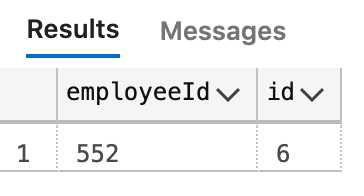
Now let's say we run the following query:
SELECT employeeId, id
FROM [dbo].[Users]
WHERE employeeId = 552
This query will be processed by a table scan, which we can see by looking at the execution plan.
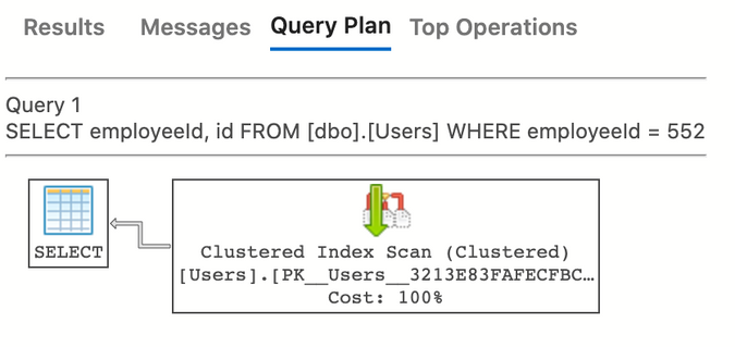
Note that while it says “clustered index scan,” it is in fact scanning the table, since the clustered index is the table, in SQL Server, for tables with a primary key defined.
The engine will simply look through each and every record, and return those which match the filter clause. This query will run blazingly fast … when there's a tiny bit of data; it will run maddeningly slow when there's a massive amount of data, and everything in between.
An index to the rescue!
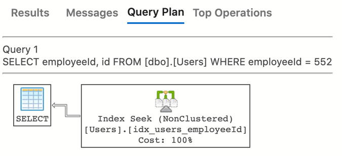
Let's say we anticipate a large amount of data in this table, and therefore want to improve this query's performance. We’d likely do so by adding an index.
CREATE INDEX idx_users_employeeId ON USERS (employeeId);
Now when we run our same query, the engine will perform a seek.
What does that mean? Let's take a very high level view of how database indexes work. They're usually stored in a data structure known as a B+ tree. There's tons of comp sci-rich resources where you can learn all about them, but for now, think of a database index like the index of a book. A book's index has an ordered list of all the terms the book has, along with a page number. Database indexes are similarly ordered based on whatever they're indexing, and contain a pointer to the page in memory where the actual record is stored (they'll also have the primary key for the record, and any "covering" fields, which we'll get to).
But a flat list of all the terms in a book is still pretty big. Nobody would ever start reading an index at aardvark, and continue on until they either found what they were looking for, or hit zebra, and with it the end of the index. Typically folks will just thumb through the pages of a book’s index, looking at the words on each page, and just sort of find what they want. But if we were to force ourselves to think about how we'd do this algorithmically, we'd probably pick the middle page of the index, look at the first, and last word listed. If our target is in between, we just start reading and find the word. If our word is less than that smallest word, we'd pick the middle page of all the pages in the first half of the index, and repeat. And of course if the word is greater than the last word on our page, we'd pick the middle page in the remaining pages in the second half of the index, and repeat. With each repetition, we'd cut the number of pages we're searching in half. That means the algorithm would run in O(lgN) time, or logarithmic complexity.
Logarithmic algorithms are incredibly fast. They're basically the inverse of exponential algorithms. Instead of a constant, like 2, multiplied by itself N times, we have N being divided by a constant repeatedly until we get to 1. That's what a logarithm means. log216, or lg16 for short, means how many times do I divide 16 by 2, until I get to 1, which is 4. To give an idea of how well logarithmic algorithms perform, note that lg of 4 billion is about 32, since 232 is about 4 billion. That's why you could never have more than 4GB of RAM on a 32 bit computer: you simply cannot create more than 4 billion unique addresses with just 32 bits.
But a real B+ tree is even better than this. Let’s dump the analogy and just look at how it works. A B+ tree is focused on getting you to the right page in memory, which contains the record you’re searching for. It starts with a root page, with a series of indexed values, with pointers to memory pages containing all values less than this value. Take this example
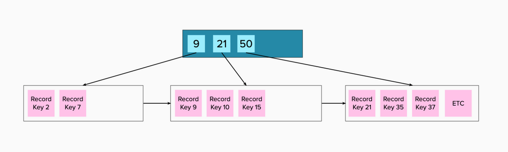
The root record is telling us that all values less than 9 are in the memory page to the left, all values less than 21 are in the middle page, and so on. The pink boxes are leaf nodes. They’ll contain the indexed value (2, 7, 9, 10, 15, 21, etc., in the picture), any covering values, which we’ll get to, and also, not shown, but a pointer to the page in memory where actual record is, as stored in the table.
These leaf pages also contain pointers to the next page, which will come in handy for range queries. For example, if you search for all values >= 10, the database engine will locate value 10, and then just walk the rest of the values in that page, then follow the pointer to the next page, consume those values, and so on. In fact, in real life those pointers between leaf pages are bidirectional, with each page containing a pointer to the next page, and also the previous page, which means an index can handle range query in either ascending or descending order.
But what happens when our table gets so big that we can no longer have a single root page with a pointer to a single memory page with all values less than a certain key. Pages in memory are a fixed size, and pointers are not free, after all. When this happens, the B+ tree will just grow, adding more non-leaf levels.
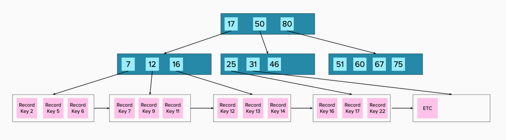
It’s the same idea as before, except now you need to load a total of three pages in memory, to get to your target, instead of two. Before we read the root, which took us right to our destination. Now we read the root, which takes us to another page of pointers, which then takes us to our destination.
Let’s see this in action. Let's say we run this query
SELECT employeeId, id
FROM [dbo].[Users]
WHERE employeeId > 3
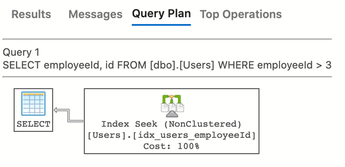
As we can see, SQL Server ran a seek to find the first value of 3, and then just kept reading the rest of the values. Cool! This query is a bit limited though. Let's also query for each user's name, and see what happens.
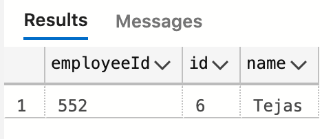
SELECT employeeId, id, [name]
FROM [dbo].[Users]
WHERE employeeId = 552
The index we added indexed on employeeId. Each leaf contains the employeeId, the primary key, and a pointer to the (page in memory containing the) full record. You might think SQL Server would do a seek on our index, then follow the pointer to the record in the table. Instead, we see this
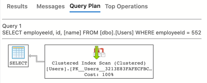
Interesting. The engine decided to just scan the main table and get what we asked for. This is almost certainly because we have a tiny amount of data in the table. SQL Server maintains metadata about the size of tables and indexes to help it make decisions like this. It also allows us to force it to use a particular index by using a “hint,” which we usually want to avoid, and let SQL Server to make smart choices for us. But just for fun, let’s see what it looks like
SELECT employeeId, id, [name]
FROM [dbo].[Users] WITH (INDEX(idx_users_employeeId))
WHERE employeeId = 552
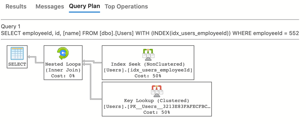
There we go. Key Lookup is the process by which SQL Server grabs the full row from the main table, and the Nested Loops is the process of combining them together.
This is what SQL Server would have done with any real amount of data, and it would kill our performance, compared to the simple seek if we were pulling back a lot of records. Before, we could seek to a particular value in a small number of page reads. But now, if our query returned 100 rows, each of those 100 rows would need to do a lookup in the main table. This latter step would dominate the performance of this query.
Without getting too deep in the weeds, we could solve this particular problem by adding what's called an "included" field. That means the index stays exactly as it is, except the "leaf" pages, which contain the indexed value, the primary key, and pointer to memory, would now also "include" whatever field(s) we add. You can include as many fields as you want, but as you do, your index grows in size. When an index can "cover" all fields a query is looking for, by some combination of the indexed fields, the primary key, and included fields, it's known as a "covering index," and will usually be quite fast.
Let’s create a new index
CREATE INDEX idx_users_employeeId_inc_name
ON USERS (employeeId) INCLUDE (name);
and re-run our query, without the hint.
Boom
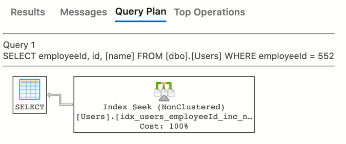
Our entire query was satisfied with a single index seek; it will scale incredibly well.
Wrapping up the theory
Thank you so much for sticking with me. The point of all this is to show that, with traditional databases, you have a wide open query language, which you combine with low level tools to try to keep your queries as fast as possible. Obviously the queries I showed were extremely simple. Usually you'll deal with joins, groupings, unions, and of course queries can specify any arbitrary sort order. When a query is slow, you'll usually look at the execution plan, see something vastly more complex than anything I've shown, find the pieces that are making things slow (table scans are usually the first thing you look for), and then try to figure out how to guide the engine into a faster query execution: add or tweak indexes, add a materialized view, add query hints, etc.
And this of course assumes that a single server will be big enough to hold all of your data. When that’s no longer is true, you'll need to "shard" your data across many different servers. Sharding is a topic unto itself. Suffice it to say, it's hard, there's a lot you have to get right, and some databases make it easier than others.
DynamoDB
Dynamo takes a fundamentally different approach. Rather than giving you a wonderfully flexible querying language, some low level indexing primitives, and wishing you luck, it's structured in such a way that you're essentially forced to make fast, scalable queries.
What follows is the high level introduction I wish I had started with, when I got interested in Dynamo. I promise I'm barely scratching the surface.
Dynamo is a NoSQL database. It enforces no schema on you, and allows you to store things like lists, and objects inside individual fields. But please don't be fooled into thinking it's like most other NoSQL databases. MongoDB has a lot more in common with SQL Server, than it does with Dynamo, and that was true even before Mongo added joins and transactions.
When you create a table in Dynamo, you'll define a Partition Key. It's sort of like a primary key in other databases, except it doesn't uniquely identify a record (assuming there’s a sort key; stay tuned). What it does is uniquely identify a list of records, which will be differentiated, and ordered by the sort key. The sort key is optional, and if you don't create one, the partition key will be exactly like a traditional primary key; but as we'll get into, you'll usually define both.
When we want to read data from Dynamo, we always (for the most part), start with the partition key. That will give you all of the rows defined with that key, ordered by the sort key (you can reverse this order in your query if you want). The best analogy I've heard is that each partition is basically a filing cabinet drawer, containing a bunch of related records. What's especially important here is that Dynamo guarantees that finding an individual partition is always fast. Basically, Dynamo comes sharded, out of the box, by partition key. This is a key point. As I said before, sharding becomes essential when your data scales, and is usually difficult to get right. But Dynamo comes with sharding out of the box, based on the partition key you define.
But we can also also filter down the records from the partition (or filing cabinet drawer) if we want. We can run filters on the sort key as well, with things like equality, less than, greater than, between, etc. It turns out that each individual Dynamo partition is stored as a ... wait for it... B+ tree. This means finding a specific value in your partition is fast.
What's especially important is what you cannot do. You cannot tell Dynamo to sort your query by some random field. You cannot join two tables, or even partitions together. You cannot do groupings. Etc. You can grab one precise value by specifying a partition key, and sort key, or you can grab a range of values within a partition, filtered by the sort key. I'll note that while you can also filter by arbitrary (non-key) fields, relying on this for major work is a strong anti-pattern. Dynamo is charging you (literally) based on how much you read, and arbitrary, non-key filters occur after the reads happen. Also, these arbitrary filters are applied after your pagination values are applied, which means they won’t work well with pagination. Dynamo is pushing you very strongly toward using key-based filters.
Again, Dynamo is extremely controlling, and specific about how it expects you to use it. Your data need to be modeled in such a way that your use cases can be satisfied by querying into a specific partition, based on sort key.
Before moving on I'll briefly note that Dynamo does allow you to scan the entire table, but there's no way to sort the results, and again, this should not be used for normal querying (unless you want your queries to be slow, and to jack up your AWS bill in the process).
Modeling Data with Dynamo
Ok so we want to design our data so that it fits into partitions, defined by the partition key, which can be further refined by the sort key. Let's see what that actually means. Let's say we wanted to create a table for books. What will each partition contain? Well, we'll need info about the book itself, we'll want records for each author, and let's also store some reviews the book received. Here's one way (among many) we could model this.
We'll name our partition key, pk, and we'll name our sort key sk. These keys should have non-descriptive, generic names. They do not represent actual aspects of books, authors, or reviews, but rather are arbitrary values we'll use to rack and stack our data in exactly a way that Dynamo will like. To be crystal clear, each Dynamo partition will contain different types of data. If you’re used to SQL Server tables, or Mongo collections each storing a single entity type, this may be a radical change for you. These Dynamo partitions contain different types of entities. That’s why our pk and sk above are generic, and detached from our domain model.
Let's say that for any book, the partition key will be Book#<isbn>. Again, we’re using this instead of just the isbn alone because with Dynamo, we’re storing many different types of data inside of the same table. Your entire project would likely be stored inside of a single table, organized by partition. If our books are keyed as Book#978111, then a publishing house might be keyed as Publisher#Random House, a book seller might be keyed as Seller#Amazon, etc. Rather than having multiple tables, each with one type of thing, we have one big table, partitioned into different types, based on the partition key.
So what kind of values will we have within each Book partition? Let's say we'll have an entry with a sort key of Metadata holding info about the book, any number of authors entries, with sort keys of Author#<name>, and any number of Review#<id> entries for the book's reviews.
Let's see what it might look like for one book:
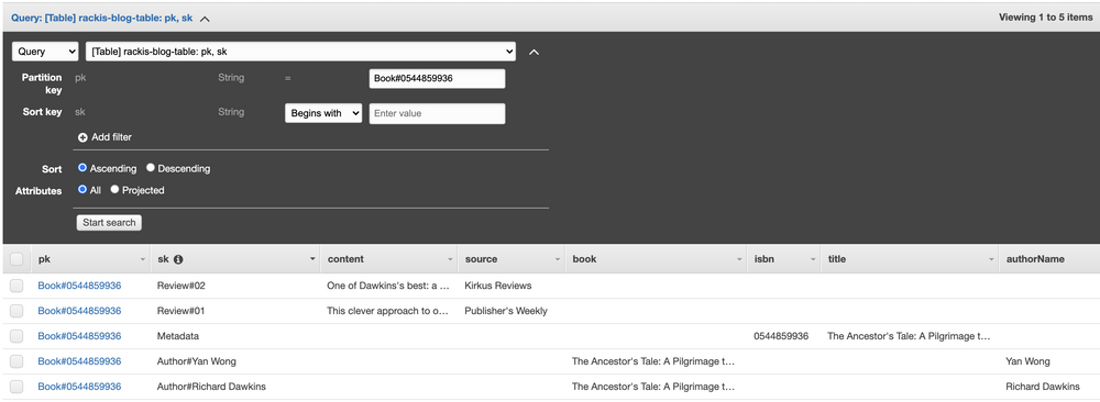
So if we want to just dump everything about The Ancestor’s Tale, we would pull that partition.
More interestingly, if we want to pull the authors of a book, we pull that partition, and further filter based on sort key values that starts with Author#.
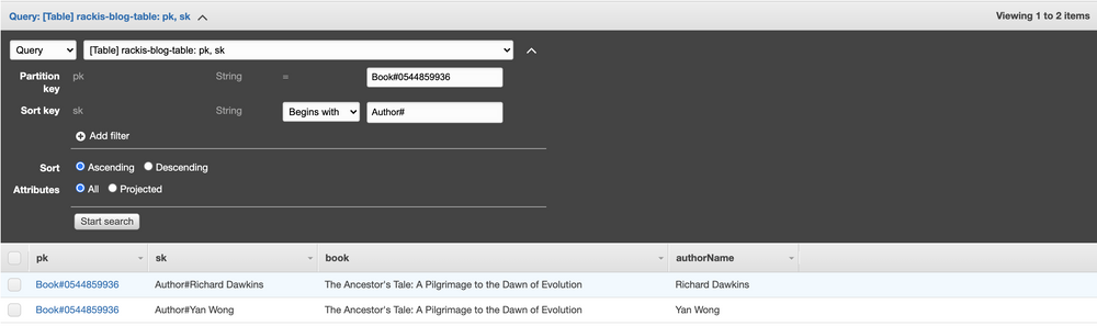
But what if we want to query a specific author, say, Richard Dawkins, and get all of their books? Things aren't looking good. Any query has to start with a partition key, but each separate book is its own partition. We definitely don't want to just scan the entire table, looking for items with a sk of Author#Richard Dawkins; that would be slow, and expensive.
Hello, GSI
One of the most important, and powerful features of Dynamo are global, secondary indexes, or GSIs. A GSI allows your to take your table, and basically project a brand new table from it, with a brand new partition, and sort key. As you update the table, the index will update automatically. Best of all, the GSI can be queried directly, just like the main table, in exactly the same way.
Let's get started. Let's build a GSI with authorName as the partition key, and book as the sort key. I'm simplifying a bit here; usually you should create and maintain dedicated fields for index keys, rather than reuse fields from your model. The reason is, if some other entity type got added to our table with an authorName field, it would pollute our index. But for this blog post, it's good enough.
What this index will do is take the items in our main table, and for those with an authorName field, a corresponding partition will be created in our index, with a sort key of book. It looks like this.
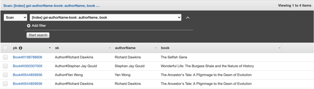
Don’t be fooled by the pk and sk fields. We projected all fields from the original table (which includes pk and sk), with a partitionKey of authorName, and a sortKey of book.
Now if we want to see Richard Dawkins's books, we can query the GSI directly.
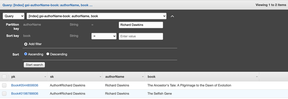
Best of all, this query is always guaranteed to be fast. Our GSI is partitioned by authorName, and again, Dynamo guarantees fast lookups on partitions. We sacrifice a lot of flexibility using Dynamo, but we gain fast, scalable queries.
What can Dynamo not do?
As we've seen, Dynamo expects us to model our data pretty precisely, for queries we plan ahead, and model for. It is not for flexible querying. If you have use cases which demand flexible, user driven queries and sorting, Dynamo might not be the best for that use case. The good news is, nobody ever said you should use Dynamo for everything. There are lots of databases out there, each with their own pro's and con's. Pick the right ones for your project.
Parting Thoughts
When I say we've only scratched the surface of Dynamo, I mean it. As I've said, the best learning resource on the market for Dynamo is Alex DeBrie's DynamoDB book. It's well over 400 pages, and there's no fluff. There are entire chapters dedicated to modeling relationships, like our authors and books, above; the structure I picked is one option among many, which I mainly picked to help highlight how GSI's work.
I hope this post has piqued your curiosity in Dynamo. It's an incredibly exciting product, that has some impressive capabilities.